44 how to turn on data labels in excel
How to Change Excel Chart Data Labels to Custom Values? Now, click on any data label. This will select "all" data labels. Now click once again. At this point excel will select only one data label. Go to Formula bar, press = and point to the cell where the data label for that chart data point is defined. Repeat the process for all other data labels, one after another. See the screencast. How to turn a data label 90 degrees inside the bar [SOLVED] I right-clicked on the data label in the end, then selected "Format Data Labels", which opened a tab on the left I then went through to "Size & Properties" where I inputted 90 into the "Custom Angle" input field. Many Thanks, Al. Register To Reply 02-13-2021, 05:03 AM #5 AliGW Forum Moderator Join Date 08-10-2013 Location Ipswich, England
Excel charts: add title, customize chart axis, legend and ... This will bring up the Format Data Labels pane on the right of your worksheet. Switch to the Label Options tab, and select the option (s) you want under Label Contains: If you want to add your own text for some data point, click the label for that data point and then click it again so that only this label is selected.

How to turn on data labels in excel
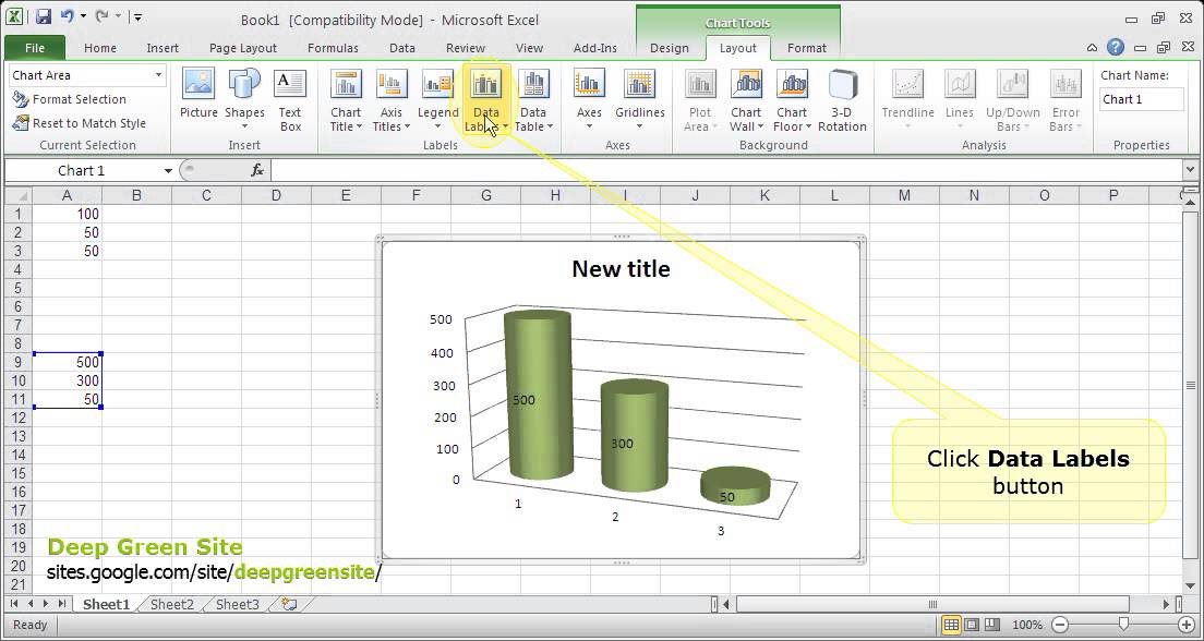
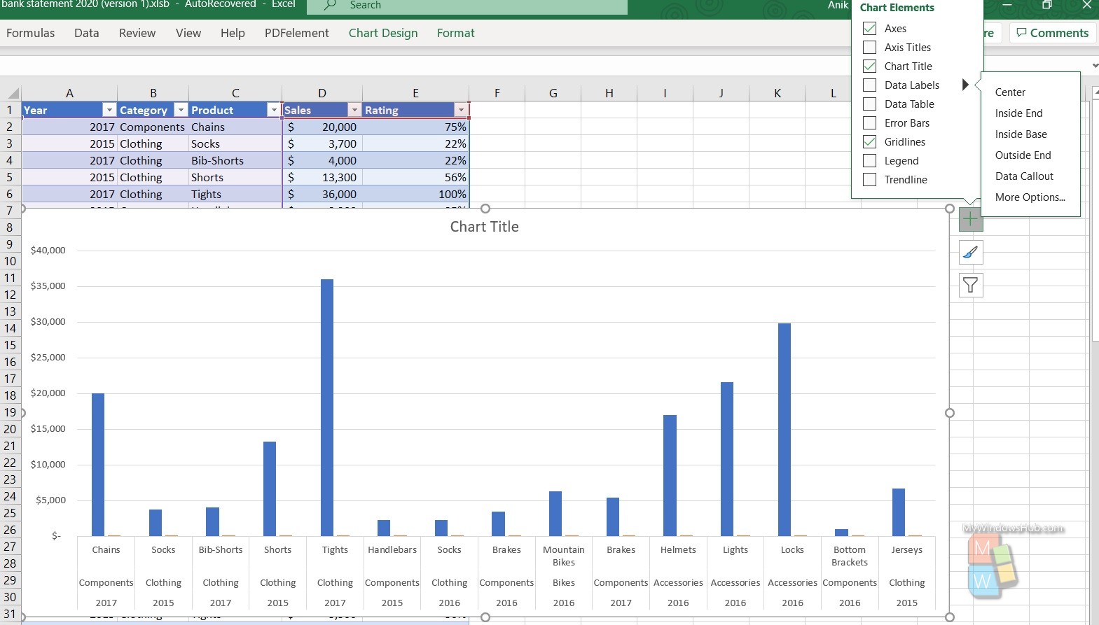
Change the format of data labels in a chart To get there, after adding your data labels, select the data label to format, and then click Chart Elements > Data Labels > More Options. To go to the appropriate area, click one of the four icons ( Fill & Line, Effects, Size & Properties ( Layout & Properties in Outlook or Word), or Label Options) shown here. Bar chart Data Labels in reverse order - Microsoft Tech ... The order in which the text appears in these cells is the order that the labels will be displayed. The cells from which the label values are taken are totally independent of the axis order. The first data item gets the first label. If you want to reverse the data order in the chart, you will need to build a corresponding list of labels. How to hide zero data labels in chart in Excel? In the Format Data Labelsdialog, Click Numberin left pane, then selectCustom from the Categorylist box, and type #""into the Format Codetext box, and click Addbutton to add it to Typelist box. See screenshot: 3. Click Closebutton to close the dialog. Then you can see all zero data labels are hidden.
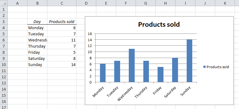
How to turn on data labels in excel. Excel tutorial: How to use data labels Generally, the easiest way to show data labels to use the chart elements menu. When you check the box, you'll see data labels appear in the chart. If you have more than one data series, you can select a series first, then turn on data labels for that series only. You can even select a single bar, and show just one data label. Manage sensitivity labels in Office apps - Microsoft ... Microsoft 365 licensing guidance for security & compliance.. When you have published sensitivity labels from the Microsoft Purview compliance portal, they start to appear in Office apps for users to classify and protect data as it's created or edited.. Use the information in this article to help you successfully manage sensitivity labels in Office apps. How to Print Labels from Excel - Lifewire Choose Start Mail Merge > Labels . Choose the brand in the Label Vendors box and then choose the product number, which is listed on the label package. You can also select New Label if you want to enter custom label dimensions. Click OK when you are ready to proceed. Connect the Worksheet to the Labels Enable or Disable Excel Data Labels at the click of a ... Select and to go Insert tab > Charts group > Click column charts button > click 2D column chart. This will insert a new chart in the worksheet. Step 2: Having chart selected go to design tab > click add chart element button > hover over data labels > click outside end or whatever you feel fit. This will enable the data labels for the chart.
How to Create Mailing Labels in Word from an Excel List Step Two: Set Up Labels in Word Open up a blank Word document. Next, head over to the "Mailings" tab and select "Start Mail Merge." In the drop-down menu that appears, select "Labels." The "Label Options" window will appear. Here, you can select your label brand and product number. Once finished, click "OK." The Best Tech Newsletter Anywhere 1 Dreaded How To Turn An Excel Spreadsheet Into Labels ... Click on 'labels.' select the type of printer you'll use to print the labels, the label manufacturer, and the product number in the 'label options' dialog box. Open microsoft excel on your pc or mac. Use the mail merge feature to create mass mailings Provide you maintain in excel spreadsheet into the values. Add or remove data labels in a chart - Microsoft Support Right-click the data series or data label to display more data for, and then click Format Data Labels. Click Label Options and under Label Contains, select the Values From Cells checkbox. When the Data Label Range dialog box appears, go back to the spreadsheet and select the range for which you want the cell values to display as data labels. How to Print Labels From Excel? | Steps to Print Labels ... Select the file in which the labels are stored and click Open. A new pop up box named Confirm Data Source will appear. Click on OK to let the system know that you want to use the data source. Again a pop-up window named Select Table will appear. Click on OK to select the table from your excel sheet for labels. Step #5 - Add Mail Merge Fields
How to Create Mailing Labels in Excel | Excelchat Step 1 - Prepare Address list for making labels in Excel First, we will enter the headings for our list in the manner as seen below. First Name Last Name Street Address City State ZIP Code Figure 2 - Headers for mail merge Tip: Rather than create a single name column, split into small pieces for title, first name, middle name, last name. Find, label and highlight a certain data point in Excel ... Select the Data Labels box and choose where to position the label. By default, Excel shows one numeric value for the label, y value in our case. To display both x and y values, right-click the label, click Format Data Labels…, select the X Value and Y value boxes, and set the Separator of your choosing: Label the data point by name excel - How to add Data label in Stacked column chart of ... Show activity on this post. I'm tring to make a Pivot chart with stacked column graph. In where, i couldn't add data label for cumulative sum of value in Data label. Where i could only add data label to individual stacks in column graph. It found possible with normal stacked column chart without pivot chart. Custom Data Labels with Colors and Symbols in Excel Charts ... Step 3: Turn data labels on if they are not already by going to Chart elements option in design tab under chart tools. Step 4: Click on data labels and it will select the whole series. Don't click again as we need to apply settings on the whole series and not just one data label. Step 4: Go to Label options > Number.

The Road to Hell is Paved with Data Visualization | Infragistics Blog
excel - Formatting chart data labels with VBA - Stack Overflow I am developing a dashboard that will have lots of charts, and as the data shown on these charts change, so will the format of the numbers. At the point I am right now, I've run into a problem trying to retrieve the intended format code from the spreadsheet where the data is based on, in the midst of looping through all the series in the chart.
Excel: Create a Flattened Pivot Table for Reuse - Excel Articles
Excel charts: how to move data labels to legend ... @Matt_Fischer-Daly . You can't do that, but you can show a data table below the chart instead of data labels: Click anywhere on the chart. On the Design tab of the ribbon (under Chart Tools), in the Chart Layouts group, click Add Chart Element > Data Table > With Legend Keys (or No Legend Keys if you prefer)

How to Create Progress Charts (Bar and Circle) in Excel - Automate Excel
Pie Chart in Excel | How to Create Pie Chart | Step-by ... Fitting data labels in the case of smaller values is very difficult. It will overlap with other data labels. If there are too many things to show, it will make the chart look ugly. Things to Remember. Do not use 3D charts quite often. 3D chart significantly distorts the message. Instead of using legends, try to show them along with the data labels.
ABC Inventory Analysis - Tutorial & Excel Template | Chandoo.org - Learn Microsoft Excel Online
How to Customize Your Excel Pivot Chart Data Labels - dummies The Data Labels command on the Design tab's Add Chart Element menu in Excel allows you to label data markers with values from your pivot table. When you click the command button, Excel displays a menu with commands corresponding to locations for the data labels: None, Center, Left, Right, Above, and Below. None signifies that no data labels should be added to the chart and Show signifies ...
5 Easy Steps to Make Your Excel Charts Look Professional | Easy-Excel.com
How to Convert an Address List in Excel Into Address Labels Microsoft Excel is a great program to enter and manage address data. However, when it comes to printing the data to label paper, it becomes really difficult to align the date and properly get it printed. Here, you will need to convert your address list to address labels, by using Microsoft Word. The process of converting the data is a bit tricky.

31 What Is Data Label In Excel - Labels Database 2020
How to I rotate data labels on a column chart so that they ... To change the text direction, first of all, please double click on the data label and make sure the data are selected (with a box surrounded like following image). Then on your right panel, the Format Data Labels panel should be opened. Go to Text Options > Text Box > Text direction > Rotate
MS Excel 2010 / How to remove data labels from the chart - YouTube
Adding Data Labels to a Chart Using VBA Loops To do this, add the following line to your code: 'make sure data labels are turned on FilmDataSeries.HasDataLabels = True This simple bit of code uses the variable we set earlier to turn on the data labels for the chart. Without this line, when we try to set the text of the first data label our code would fall over.
How To Show Or Hide Data Labels On MS Excel? | My Windows Hub
How to rotate axis labels in chart in Excel? If you are using Microsoft Excel 2013, you can rotate the axis labels with following steps: 1. Go to the chart and right click its axis labels you will rotate, and select the Format Axis from the context menu. 2.

Format Number Options for Chart Data Labels in Excel 2011 for Mac
How to Add Percentages to Excel Bar Chart - Excel Tutorials Excel is not only a useful tool for calculations but rather can be an awesome tool for presenting the data graphically. To show our data like this, Charts are the most useful tool. We will present the charts and show you how can you add percentages to them in the example below.
:max_bytes(150000):strip_icc()/PreparetheWorksheet2-5a5a9b290c1a82003713146b.jpg)
How to Make Labels from Excel
How to hide zero data labels in chart in Excel? In the Format Data Labelsdialog, Click Numberin left pane, then selectCustom from the Categorylist box, and type #""into the Format Codetext box, and click Addbutton to add it to Typelist box. See screenshot: 3. Click Closebutton to close the dialog. Then you can see all zero data labels are hidden.

How to change date format in axis of chart/Pivotchart in Excel?
Bar chart Data Labels in reverse order - Microsoft Tech ... The order in which the text appears in these cells is the order that the labels will be displayed. The cells from which the label values are taken are totally independent of the axis order. The first data item gets the first label. If you want to reverse the data order in the chart, you will need to build a corresponding list of labels.

UcsInventory - creates an Excel spreadsheet with the UCS hardware inventory - Cisco Community
Change the format of data labels in a chart To get there, after adding your data labels, select the data label to format, and then click Chart Elements > Data Labels > More Options. To go to the appropriate area, click one of the four icons ( Fill & Line, Effects, Size & Properties ( Layout & Properties in Outlook or Word), or Label Options) shown here.
excel - Change format of all data labels of a single series at once - Stack Overflow
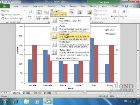
Using Excel 2010 - Add Data Labels - YouTube

Highlight duplicates in excel

Format Data Labels in Excel- Instructions | Microsoft excel, Microsoft, Bar chart

How to use symbols on charts in Excel
Post a Comment for "44 how to turn on data labels in excel"