44 google sheets horizontal axis labels

How to Make a Scatter Plot in Google Sheets (Easy Steps) Display the x or y-axis as labels rather than numeric values. How to Do a Scatter Plot in Google Sheets with Different Gridlines and Ticks This category lets you format the scatter chart to contain major and/or minor gridlines. How do I change the Horizontal Axis labels for a line chart in Google ... I am trying to create a line chart in google docs, I want to have the horizontal axis separated into dates with weekly intervals, I cant seem to find where to set the labels for the horizontal axis. I'm happy with everything else so far but the labels don't match up with the data I have.

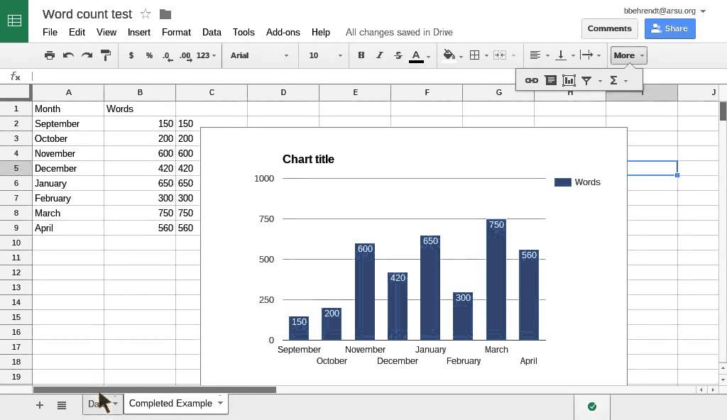
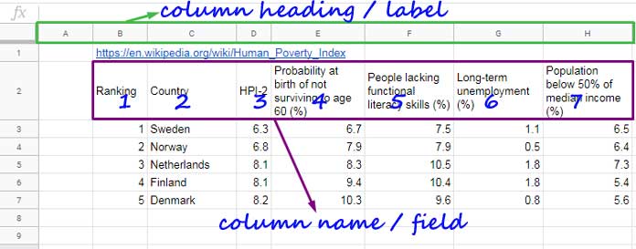
Column charts - Google Docs Editors Help Labels from the first column show up on the horizontal axis. First row (Optional): In the first row of each column, enter a category name. Entries in the first row show up as labels in the legend. Other columns: For each column, enter numeric data. You can also add a category name (optional). Other cells: Enter the data points you’d like to ...

Google sheets horizontal axis labels

Controls and Dashboards | Charts | Google Developers Jul 07, 2020 · 'horizontal' Whether the label should display above (vertical stacking) or beside (horizontal stacking) the category picker. Use either 'vertical' or 'horizontal'. ui.cssClass: string 'google-visualization-controls-categoryfilter' The CSS class to assign to the control, for custom styling. How to Add a Horizontal Line to a Chart in Google Sheets How to Add a Horizontal Line to a Chart in Google Sheets Occasionally you may want to add a horizontal line to a chart in Google Sheets to represent a target line, an average line, or some other metric. This tutorial provides a step-by-step example of how to quickly add a horizontal line to a chart in Google Sheets. Step 1: Create the Data Google Workspace Updates: New chart axis customization in Google Sheets ... New chart axis customization in Google Sheets: tick marks, tick spacing, and axis lines Monday, June 29, 2020 Quick launch summary We're adding new features to help you customize chart axes in Google Sheets and better visualize your data in charts. The new options are: Add major and minor tick marks to charts. ... Labels: Editors ...

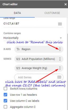
Google sheets horizontal axis labels. Change axis labels in a chart - support.microsoft.com On the Character Spacing tab, choose the spacing options you want. To change the format of numbers on the value axis: Right-click the value axis labels you want to format. Click Format Axis. In the Format Axis pane, click Number. Tip: If you don't see the Number section in the pane, make sure you've selected a value axis (it's usually the ... How do I format the horizontal axis labels on a Google Sheets scatter ... Make the cell values = "Release Date" values, give the data a header, then format the data as YYYY. If the column isn't adjacent to your data, create the chart without the X-Axis, then edit the Series to include both data sets, and edit the X-Axis to remove the existing range add a new range being your helper column range. Share Improve this answer How to Make a Line Graph in Google Sheets - 4 Simple Methods Below are the steps to create a line combo chart in Google Sheets: Select the dataset. In the toolbar, click on the 'Insert chart' icon (or go to the Insert option in the menu and then click on Chart). At this point, your chart may look something as shown below. Google Sheets Horizontal Axis Label: Filter value? - Google Docs ... This help content & information General Help Center experience. Search. Clear search

Text-wrapping horizontal axis labels - Google Groups The labels for the horizontal axis are linked to text alongside the calculations for the charts. The text in the labels is of varying lengths and for some of the charts, this text is being wrapped... How to create a chart in Excel from multiple sheets ... Nov 05, 2015 · Make a chart from multiple Excel sheets; Customize a chart created from several sheets; How to create a chart from multiple sheets in Excel. Supposing you have a few worksheets with revenue data for different years and you want to make a chart based on those data to visualize the general trend. 1. Create a chart based on your first sheet How to make a 2-axis line chart in Google sheets - GSheetsGuru In order to set one of the data columns to display on the right axis, go to the Customize tab. Then open the Series section. The first series is already set correctly to display on the left axis. Choose the second data series dropdown, and set its axis to Right axis. Step 5: Add a left and right axis title How to Add Axis Labels in Google Sheets (With Example) Step 3: Modify Axis Labels on Chart. To modify the axis labels, click the three vertical dots in the top right corner of the plot, then click Edit chart: In the Chart editor panel that appears on the right side of the screen, use the following steps to modify the x-axis label: Click the Customize tab. Then click the Chart & axis titles dropdown.

Customizing Axes | Charts | Google Developers For line, area, column, combo, stepped area and candlestick charts, this is the horizontal axis. For a bar chart it is the vertical one. Scatter and pie charts don't have a major axis. The minor... How to Switch Chart Axes in Google Sheets - How-To Geek To change this data, click on the current column listed as the "X-axis" in the "Chart Editor" panel. This will bring up the list of available columns in your data set in a drop-down menu. Select the current Y-axis label to replace your existing X-axis label from this menu. In this example, "Date Sold" would replace "Price" here. How to LABEL X- and Y- Axis in Google Sheets - YouTube Subscribe How to Label X and Y Axis in Google Sheets. See how to label axis on google sheets both vertical axis in google sheets and horizontal axis in google sheets easily. In addition, also see... Move Horizontal Axis to Bottom - Excel & Google Sheets Click on the X Axis Select Format Axis 3. Under Format Axis, Select Labels 4. In the box next to Label Position, switch it to Low Final Graph in Excel Now your X Axis Labels are showing at the bottom of the graph instead of in the middle, making it easier to see the labels. Move Horizontal Axis to Bottom in Google Sheets

35 How To Label Horizontal Axis In Google Sheets - Labels Information List

How To Add Axis Labels In Google Sheets in 2022 (+ Examples) Step 4. Go back to the Chart & Axis Titles section above the series section, and choose and click on the dropdown menu to select the label you want to edit. This time, you'll see an additional menu option for Right Vertical Axis Title. Click on it.

32 How To Label The Legend In Google Sheets - 1000+ Labels Ideas

How to slant labels on the X axis in a chart on Google Docs or Sheets ... How do you use the chart editor to slant labels on the X axis in Google Docs or Google Sheets (G Suite)?Cloud-based Google Sheets alternative with more featu...

How to make a 2-axis line chart in Google sheets | GSheetsGuru

Chart Axis – Use Text Instead of Numbers – Excel & Google Sheets Change Labels. While clicking the new series, select the + Sign in the top right of the graph; Select Data Labels; Click on Arrow and click Left . 4. Double click on each Y Axis line type = in the formula bar and select the cell to reference . 5. Click on the Series and Change the Fill and outline to No Fill . 6.

Common Errors in Scatter Chart in Google Sheets That You May Face

How to Insert Axis Labels In An Excel Chart | Excelchat Add label to the axis in Excel 2016/2013/2010/2007. We can easily add axis labels to the vertical or horizontal area in our chart. The method below works in the same way in all versions of Excel. How to add horizontal axis labels in Excel 2016/2013 . We have a sample chart as shown below; Figure 2 – Adding Excel axis labels

Google Chart: How to draw the vertical axis for LineChart? - Stack Overflow

How to Add Axis Labels to a Chart in Google Sheets Step 1: Double-Click on a blank area of the chart. Use the cursor to double-click on a blank area on your chart. Make sure to click on a blank area in the chart. The border around the entire chart will become highlighted, and the Chart Editor Panel will appear on the right side of the page. The Chart Editor Panel is where you will make changes ...

Show Month and Year in X-axis in Google Sheets [Workaround]

Make a Google Sheets Histogram - An Easy Guide for 2022 Slant labels to display the axis labels at a particular angle. For example, you might want to display the labels at an angle of 90 degrees from the horizontal axis as shown below. Your histogram would then look like this: Gridlines and Ticks Finally, you can format the histogram to contain major and/or minor gridlines.

31 Label Columns In Google Sheets - Modern Labels Ideas 2021

Show Month and Year in X-axis in Google Sheets [Workaround] Essential Column Chart Settings Related to Monthly Data Under the "Customize" tab, click on "Horizontal axis" and enable (toggle) "Treat labels as text". The Workaround to Display Month and Year in X-axis in Sheets First of all, see how the chart will look like. I think it's clutter free compared to the above column chart.

35 How To Label Horizontal Axis In Google Sheets - Labels Information List

How to Change Horizontal Axis Values - Excel & Google Sheets How to Change Horizontal Axis Values in Google Sheets Starting with your Graph Similar to what we did in Excel, we can do the same in Google Sheets. We'll start with the date on the X Axis and show how to change those values. Right click on the graph Select Data Range 3. Click on the box under X-Axis 4. Click on the Box to Select a data range 5.

Share :